Using ArcPro and UAS data to Calculate Impervious Surface Area

Introduction

  The purpose of this lab is use ArcPro to create a map showing impervious surface areas for a select neighborhood near Louisville Kentucky. This will be done by following the Esri tutorial Calculate Impervious Surfaces from Spectral Imagery. This tutorial consists of using given UAS data to segment the imagery, to classify land cover types between pervious and impervious, and to calculate the impervious surface area. One goal of this lab is to summarize the tutorial and the steps that were needed to make the map. The second goal is to display and describe the patterns on the map based off of the calculated data.

Methods

Lesson 1: Separate Bands and Segment the Imagery

  This consisted of extracting the spectral bands from the aerial image. The image was separated into three bands: near infrared, red, and blue. Near infrared bands emphasize vegetation, red bands emphasize human-made objects and vegetation, and blue bands emphasize water bodies. A screen shot of the result is shown in figure 4.0 below.

Fig 4.0: Screenshot of extracted bands

Fig 4.1: Segment Mean Shift on the fly

   The second part of the lesson was about segmenting the image. Doing this will group pixels with similar characteristics. This helps to standardize the image while making it easier to work with. The Segment Mean Shift on the Fly tool was used to do this. The parameters can be seen on the right in figure 4.1. However, doing this contained some errors in the image, so the Segment Mean Shift tool was used to fix it. The input raster Extract Bands was used in the input raster box and the output was saved as Louisville_Segmented.tif. Doing this resulted in a simpler image which makes it easier to classify areas. This .tif can be seen below in figure 4.2.

Fig 4.2: Segment Mean Shift Output Raster

Lesson 2: Classifying the Raster

  This lesson started out with using the Image Classification toolbar to access the Training Sample Manager to classify different surfaces. Rectangles were drawn on the roofs, roads, driveways, grass, bare-earth, water, and shadows. Each rectangle contained only one pixel color. Many rectangles were drawn on the image and were given the proper classification. This can be seen in the screenshot below in figure 4.3. These training samples were then saved as a separate shapefile.

Fig 4.3: Classifying Data

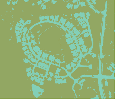
  Next, the Classify Raster tool was used to use the training sample classifications an apply them to the image of the neighborhood as a whole. After doing this raster was classified with the things specified in the Training Sample Manager. After that, the raster/aerial image was reclassified into two distinct categories: impervious, and pervious. The gray roofs, roads, and driveways were grouped as impervious, and bare earth, grass, water, and shadows were grouped as pervious. The result is displayed below in figure 4.4. The blue represents the impervious area and the green represents the pervious area.

Fig 4.4: Pervious vs Impervious Surface Area

Lesson 3: Calculating the Impervious Surface Area.

    First, this new generalized image in figure 4.4 was compared to the original aerial image. This was done by creating a series of accuracy assessment points. These points are displayed on the image shown in figure 4.4, but reflect the original image in their attributes. A total of 100 random points were generated using a equalized stratified random sampling technique. This result is shown below in figure 4.5.

Fig 4.5: Sample Accuracy Points

  Next, the attributes of these points were examined to see if there any errors in the raster. Some errors had to be fixed, but most of data was correct. Only 10 points were examined, just for practice. Luckily, Esri already had a feature class which contained an accuracy assessment points which will be used for the rest of this tutorial. This saves tedious work as examining 100 points would take a while.

  A confusion matrix was created to also see the accuracy of the raster. This is a way to test the users accuracy when examining the data. If a low percentage is displayed in the new field, then it is likely that the user didn't do a good enough job when creating the training samples shapefile. For this tutorial, a user accuracy of 94% and a producer accuracy of 98% were calculated. The Kappa accuracy was 92%. Kappa accuracy is a combination between the users and the producers accuracy. A Kappa accuracy below 85% - 90% suggests that the training samples should be recreated. 

  Finally, the impervious area of the parcels is ready to be calculated. This is done by using the Tabulate the Area tool. The Parcels feature class was used as the input zone and the zone field was set to Parcel_ID. The raster displayed in figure 4.4 was used as the input raster. The output table was set to Impervious_Area, and the cell processing size was set to .5. To complete the calculation, a join was performed between this new output table (Impervious_Area) and the Parcels feature class using Parcel_ID as the common key. After this, the data was ready to mapped.

Results/Discussion

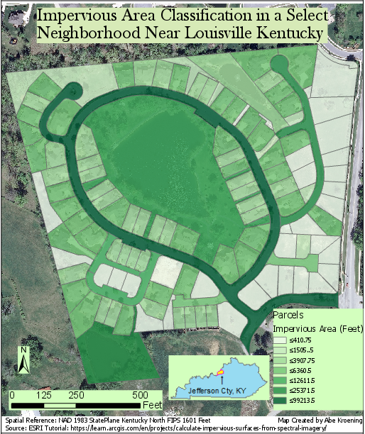
  The map below in figure 4.6 classifies the parcels by total impervious area. Parcels with greater impervious area are shown in dark green while parcels with less impervious area are shown in light green. The map was given a slight transparency so that some features beneath the parcel feature class could be seen. Generally, the least impervious parcels are located in eastern part of the map where there are no structures or roads. Most parcels west of this contain houses. The impervious area in these parcels tends to be randomly distributed. It is clear that the streets are the most impervious parcels in the image. Parcels which contain pavement, or roofs contain more impervious surface area than parcels which don't contain these. The center parcel, where the pond is located has a higher impervious area than some of the parcels which have roofs and driveways. This is because this data isn't standardized which makes large parcels more likely to have more impervious area just because of their size. This can be most easily identified when looking at the two different street parcels. Because the west street parcel has a larger area, than the east street parcel, it contains more impervious area even though the surfaces in both parcels are the same. The reason the data wasn't standardized is because storm water fees are usually based off of total runoff, not the percentage of impervious area. 

Figure 4.6: Impervious Area Map

Conclusion

  In conclusion, UAS data is well suited to be used to calculate impervious surface area. The calculations done in this tutorial could potentially be used by local governments to help decide storm water runoff fees by parcel. Similar analysis could be done on past raster imagery and then could be compared to current imagery. By doing this, one could calculated the change in impervious surface area for a certain location over period of time. Because this tutorial only used the parcels feature class and aerial imagery raster, this analysis could be done on a much larger scale. Doing this on a larger scale would help to create more spatial patterns in the map. UAS imagery can be very accurate which helps with the accuracy of calculating impervious area. Besides local government, the DNR office and the general public may be interested in this type of assessment. A good amount of storm runoff runs into lakes and streams, and by doing analysis such as in this tutorial, one could calculate this amount.
  ArcPro is the future of working with geospatial data. In just a few years ArcPro will become the standard software which people will expected to know how to use in the geospatial field, just like ArcMap is now. Becoming accustomed to using ArcPro now will be very beneficial in the future.

Sources

Esri, Learn ArcGIS, Calculate Impervious Surfaces from Spectral Imagery

  https://learn.arcgis.com/en/projects/calculate-impervious-surfaces-from-spectral-imagery/